Contact Us
CiiS Lab
Johns Hopkins University
112 Hackerman Hall
3400 N. Charles Street
Baltimore, MD 21218
Directions
Lab Director
Russell Taylor
127 Hackerman Hall
rht@jhu.edu
Last updated: 05/08/2020 5.49 pm
Our project aims to simulate and calibrate the Galen surgical platform. We will first create a virtual model and simulation for the Galen to have a safe and accessible environment for testing trajectories and software. We will then simulate a calibration experiment to test our developed calibration pipeline. Due to the COVID-19 lockdown, we currently don't have access to the Galen robot to calibrate it. However, the pipeline is ready to be used with the real robot when researchers regain access to the Galen robot, and can be used to perform the real-world experiment on the robot to improve its end effector accuracy.
The Galen platform is a family of hand-over-hand, collaborative robots developed in the Johns Hopkins Laboratory for Computational Sensing and Robotics. Intended for hand tremor cancellation in a broad range of surgical procedures, it is currently being commercialized by Galen Robotics, a robotics startup in Baltimore, MD.
Galen features a custom five degree of freedom architecture, and covers the footprint of about one person in the operating room. A wide variety of tools can be attached to the Galen for the surgeon to operate with such as pointers, drills, and forceps. While the surgeon operates with these tools, the Galen steadies their hand and cancels any tremor which can complicate the surgical procedure.
Since it’s intended to help with delicate movement such as tremor, and since the nature of surgical operations is sensitive with very small error tolerances, the Galen platform needs to be a high precision and accuracy robot, which calls for an accuracy assessment and kinematic calibration for improvement. In addition to calibrating the real-world robot, a virtual simulation of the Galen robot would be beneficial for testing and debugging control software, kinematic and dynamic parameters, and trajectories by providing a safer and much more available and accessible environment for experimentation.
Therefore, in this project we aim to:
1- Develop a calibration software pipeline that corrects for systematic errors in the Galen Mk. 2.
2- Develop a calibration simulation model representative of a live calibration experiment with the Galen Mk. 2.
3- Verify our calibration pipeline by testing it on calibration data from the Galen Mk. 2 simulation model.
Note: While our project submission includes all of the above material, our actual submission to Galen Robotics will be structured a bit differently and will include additional material. In addition to the project files, which will be given to Galen Robotics via access to a private BitBucket repo, we will also be granting Galen access to Nico's public GitHub page where they will be able to clone the forked version of AMBF used to run the Galen simulation models. We aim to do this hand-off following finals period.
Simulation model: The Galen Mk. 2 simulation is an environment where employees and research affiliates can manipulate a physically accurate model of the Galen Mk. 2 platform. The simulation will be developed in Blender animation studio and will utilize the Asynchronous Multi-Body Framework (AMBF) software package, an open source toolbox for real-time dynamic modeling of rigid bodies. Galen Robotics has provided 3D mesh files of the robot that will be imported into the simulation environment. We are currently working on producing video tutorials showing how to work with the simulated robot and run calibration trajectories with it. These tutorials will be passed on to Galen Robotics following the submission of the project.
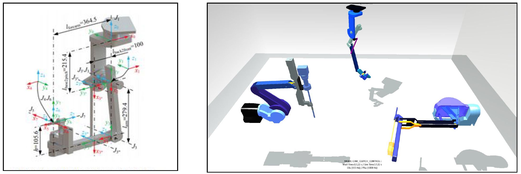 Sample virtual model of dVRK MPMs [2] (left), multiple virtual robot models in AMBF simulation environment [3] (right)
Here are pictures of the simulation model's Blender file and AMBF simulation:
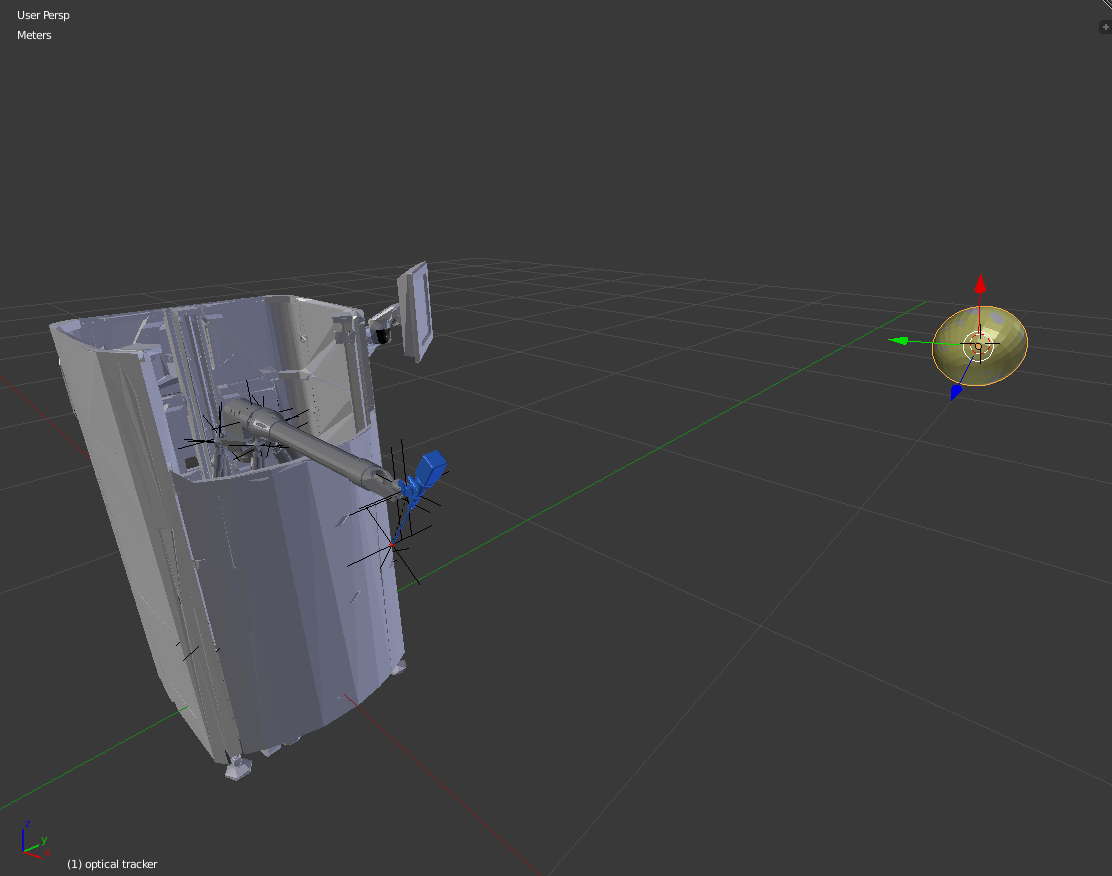 The Galen Mk.2 has been modeled in Blender Animation Studio
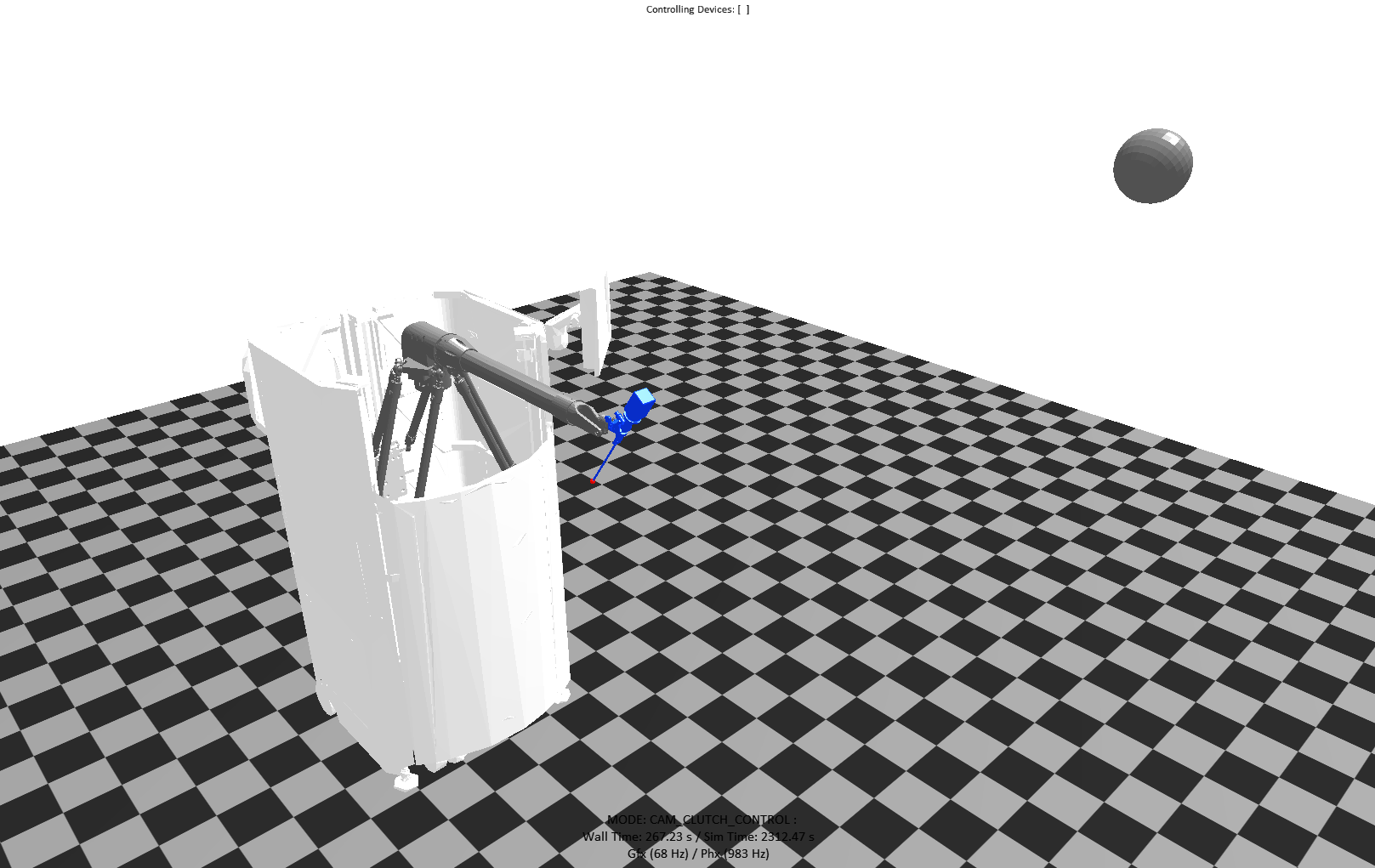 With the robot model, we can simulate its dynamics and run calibration trajectories in the AMBF simulator
Simulation control script: Users interact with the simulated robot in the AMBF simulation environment via a custom Python client, a modified version of the template client provided in the AMBF GitHub repository. The AMBF Python client provides various functions to manipulate and extract information from bodies and joints defined in the Blender model. Our final control script for our calibration simulation performs the 3 basic functions listed below:
1. Reads trajectory “.csv” file and defines arrays of desired joint values for each of the robot’s 5 actuated joints. In this way, for example, the 5th index of each array gives the joint space values corresponding to the 6th robot configuration in the trajectory.
2. Commands the robot to some preset thresholds of the desired configuration. A more detailed explanation of how these thresholds were chosen is given below.
3. Outputs the pose of the robot end-effector and optical tracker to a “.csv” file. The poses are given by AMBF in the form [x, y, z, yaw, pitch, roll].
Performance testing: In addition to building the physical simulation model and writing the control script, further steps were taken during trajectory testing to optimize the performance of the simulation robot. This mostly entailed tuning the the model's joint controller PID gains and damping coefficients. Tuning these parameters was an iterative process that included extensive “trial-and-error” testing for two different controllers: AMBF's internal controller (called directly from the “set_joint_pos()” function) and a custom controller developed with the help of Dr. Munawar. Following the advice of Dr. Munawar, we settled on using AMBF's internal controller and proceeded to tune the PID gains and damping coefficients for each joint. The figure below shows our debugging process; using ROS's PlotJuggler, we outputted the AMBF controller's commanded joint efforts and the simulation model's current joint positions while running sample trajectories. We used the plotted behavior to incrementally tweak our gains.
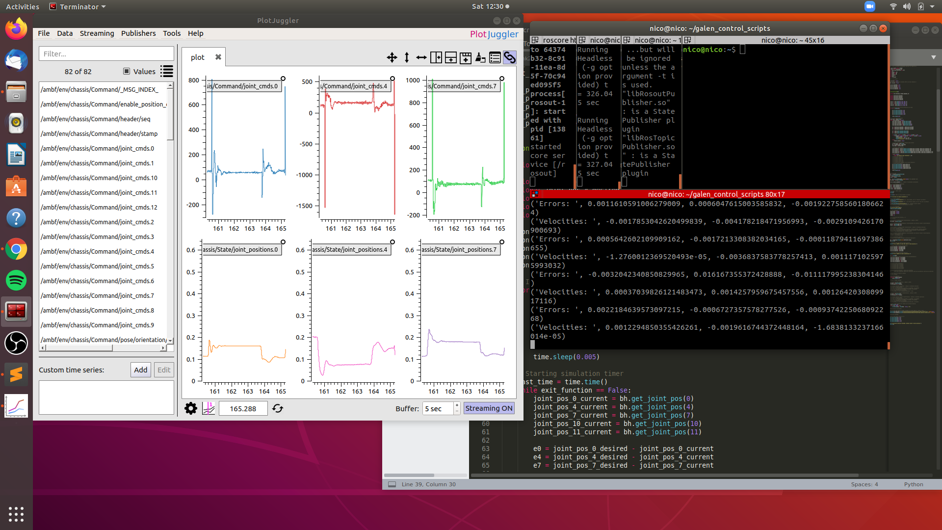 Using PlotJuggler to observe the performance of the simulation model's joint controllers and iteratively modify their PID gains and damping coefficients. This figure specifically shows us working to improve the three delta joint controllers.
The calibration procedure we implemented is based on a previous paper by Feng et. al [4] where the researchers have calibrated a predecessor to the Galen platform. They use an external optical tracker and external reference in the experimental setup, and treat the kinematics observed by the tracker as the ground truth kinematics of the system. Said kinematics are presented in Figure 7.
 Figure 7: Kinematics of the Galen Robot [4] for the calibration experiment
In this experimental setup, there are two unknown transformations: Ttip, the unknown transformation between the end effector and fiducials, and TB, the relative transformation between the robot base and the reference frame. We start the calibration protocol by solving for these unknowns, following the kinematics in Figure 7:

We can use the relationship between TB and Ttipat the initial pose (i = 0):

And substitute it into (1) and rearrange to yield:

Similarly, we can rearrange (3) into (6) and substitute into (3), rearranging again to yield:

Equations (5) and (8) have the form of an AX = XB problem. One possible way of solving this form of problems is the Park and Martin Method [5], the details of which are discussed in Appendix A: Calibration Pipeline Documentation and in our Final Project Report. Once we know Ttip and TB, we can calculate the predicted, actual transformation to the end effector from the observations of the optical tracker:

We can then compare this predicted pose to the pose acquired by the robot’s forward kinematics to calculate the pose error as:

We can express both the small error ΔKi and the distorted pose Ki in terms of the robot’s degrees of freedom, which allows us to fit a (Bernstein) polynomial that can be applied to Ki to yield a matrix of coefficients S that give correspondence between each pose and their error:

The detailed steps to calculating these coefficients can be seen in Appendix A. The fitted polynomial can then be applied to any pose in the workspace to find the correction transformation that must be added to the robot’s forward kinematics in order to result in the correct pose.

The error between this new, corrected pose and predicted can be calculated. If it is larger than desired, this new transformation can be fed back into the calibration pipeline to recalculate Ttip and TB again solving the hand-eye calibration problem, iterating until the discrepancy is sufficiently small. The workflow for the overall calibration pipeline is presented as Figure 8:
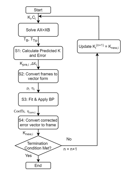 Figure 8: Calibration pipeline workflow chart
Since we have lost access to the Galen platform, we have decided to perform the calibration experiment in the virtual simulation environment using the robot model. In order to do so, two trajectories were generated to fit polynomials to, spanning the delta and work workspaces with 3000 and 1300 configurations respectively as seen in Figures A and B. Two other test trajectories covering different points inside the workspace from the fit trajectory were also generated to test how much accuracy improvement the fit polynomial actually results in.
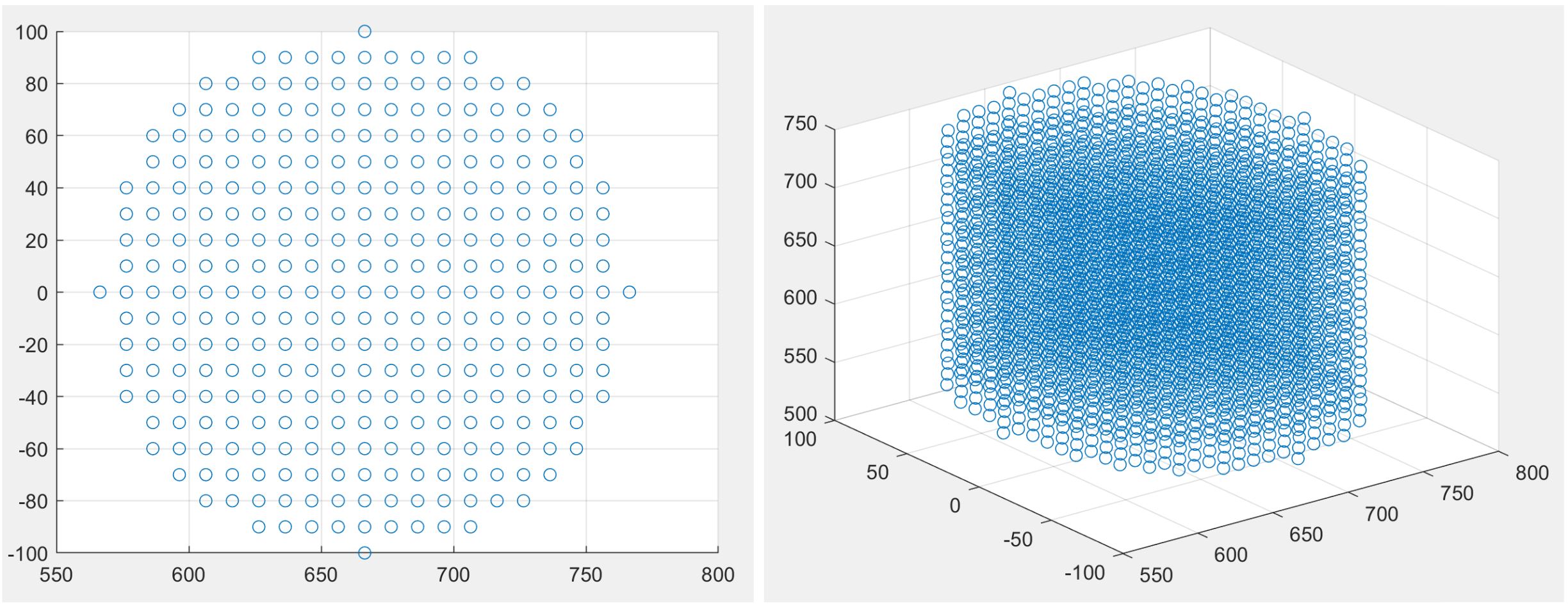 Figure 9: Delta calibration trajectory top and oblique view
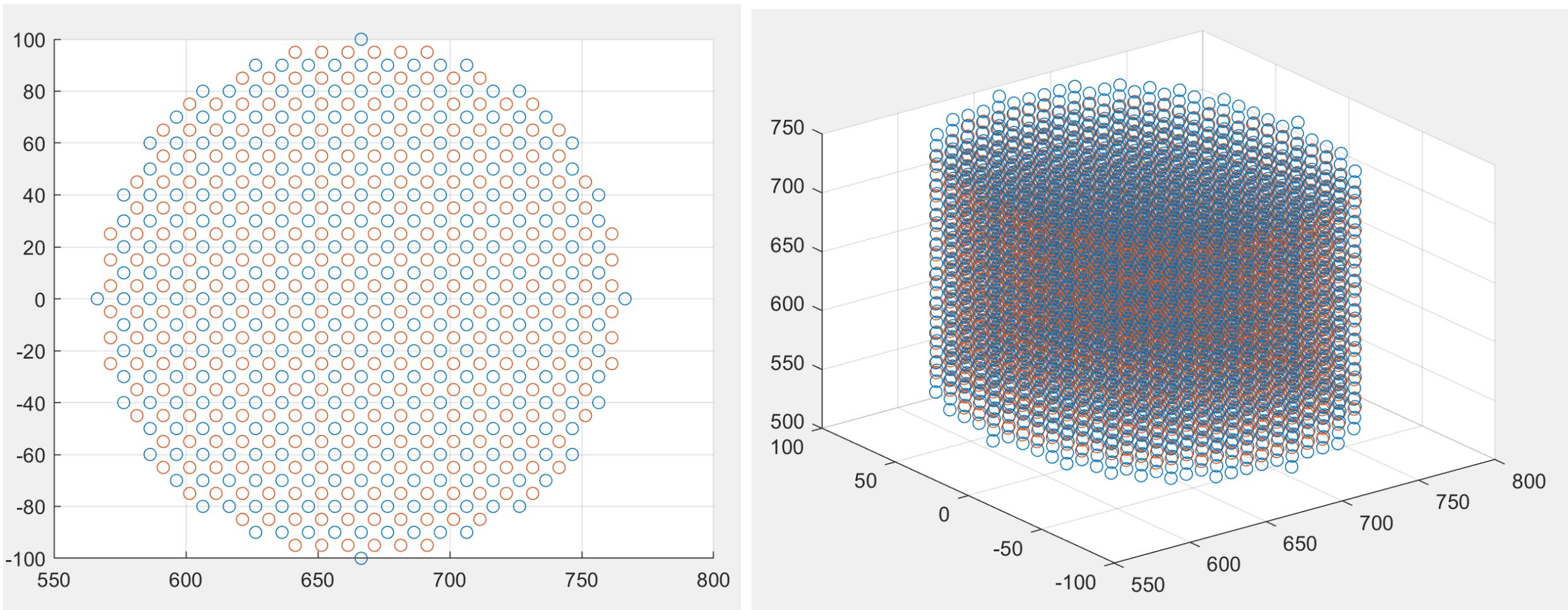 Figure 10: Delta test trajectory (red) vs calibration trajectory (blue), top and oblique view
The generated trajectories were saved into csv files with each row containing the joint configuration expected to reach each point, calculated by the inverseKinematics.m file Galen Robotics had provided. The control script reads and moves the joints to the desired configurations using a PID controller. Once the robot has sufficiently converged to the desired point, the pose of the end effector with respect to the Blender global frame, is saved and outputted to a csv file as a Cartesian position and roll-pitch-yaw. The data reading file in the calibration code reads each pose and converts it into the homogeneous transformation matrix, Ci. The data reading file also reads and passes on the joint configurations ⍴i (kdof), and from them calculates the forward kinematics for each joint configuration Ki. These transformations and vectors are then fed into the calibration pipeline, which calculates the correction function coefficients S. These coefficients are then applied to the respective test dataset containing different points in the same workspace. Positional error between K and Kpre and K and Knew are calculated and compared in the script to quantify the accuracy improvement after calibration.
Since the goal of calibration is to correct for systematic errors, three robot models with varying degrees of error were designed and tested. Though many modes of systematic error exist, we focused on two that greatly impact the Galen Mk. 2’s workspace accuracy: manufacturing errors in the length of the delta legs and minimum encoder resolution of the roll and tilt joints. See Figures # and # for visual depictions of these errors. The three robots correspond to an ideal Galen Mk. 2 model, a worst-case Galen Mk. 2 model, and a realistic Galen Mk. 2 model. Figure 11 shows the exact values of artificial systematic error injected into the models.
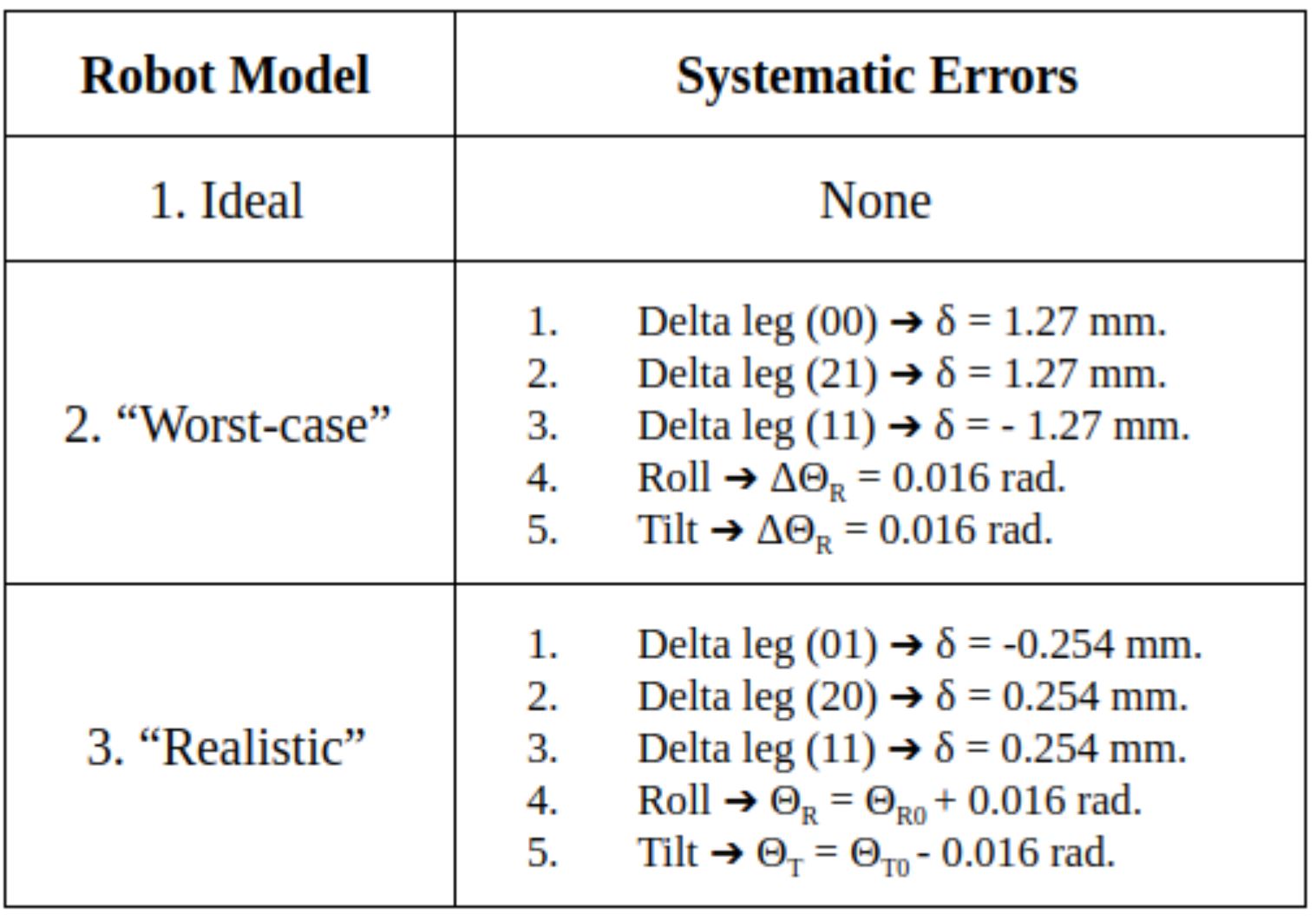 Figure 11: Systematic Errors Added to Distort the Ideal Robot
The pipeline was run with Bernstein polynomials of order 3, 4, and 5 to compare their effects. Orders 3 and 4 seemed to yield similar results, whereas order 5 was seen to overfit and therefore distort the data even further. This comparison can be seen in Table 1 for the delta stage. Since accuracy improvement from the 4th and 3rd order polynomials were very similar, we preferred to use 3rd order polynomials (for computational efficiency) to fit the different robot models with varying degrees of systematic error. The maximum and mean Euclidean position and angular errors for each robot before and after applying the correction polynomial is presented under Table 2.
The XYZ and wrist errors in the ideal robot are caused by the 0.5 mm and 0.01 rad convergence thresholds we have set up in the control script respectively, in order to have fast experiments. And although XYZ errors were already submillimeter to begin with due to small manufacturing tolerances, they are reduced even further to 0.2 mm after being corrected in the calibration process. For a visual comparison of position errors before and after calibration, Kpre is superimposed with K and Knew in Appendix C for each robot model. It should be noted that the model with the largest added errors has the highest mean error as expected before correction, however features smaller maximum XYZ error, indicating that the other models have outlier data points with higher error.
Meanwhile, angular errors in the wrist are already very miniscule to begin with around one thousandth of a radian or less, and are further improved by the correction function as expected. However, such small errors lead to the conclusion that calibrating the wrist is definitely not as much of a priority as calibrating the delta stage, as there is less room for error due to high resolution, high precision encoders and actuators in the revolute joint. The error before correction for the ideal model is in some cases slightly worse than the other models, which is due to the same 0.5 mm and 0.01 rad convergence threshold we employed for all models. In short, the correction through calibration seems to reduce inaccuracies in every case as expected, especially for the delta stage.
In this project we have developed a calibration pipeline ready to be used with the Galen Mk. 2 robot, and a virtual Galen model and simulation that is much more accessible than the robot itself. We have used the simulation to test our pipeline, and compared the effects of different modes of systematic errors on the robot model, demonstrating the usefulness of the simulation tool and that kinematic calibration using our software improves robot accuracy in both the delta stage and the wrist of the robot.
The next step for researchers continuing this project will be to test and use the calibration pipeline on the real Galen robot, and incorporate the calculated correction function in the robot’s controls in the Galen research software branch to improve its kinematic accuracy. Such increased accuracy would pave the way for new possibilities such as the implementation of virtual fixtures on the robot. Before handing over our simulation model to Galen, we also hope to make some small improvements to the simulation control script to increase its performance when running complex trajectories. While the current version is plenty fast to run the trajectories we needed for this project, trajectory interpolation and further PID tuning could make it more robust for future work.
Furthermore, more extensive studies covering a much broader range of systematic errors can be conducted on the simulated robot to identify and focus on finding solutions for the most impactful modes of error. Perhaps most importantly, this simulation environment and model robot can be duplicated very easily on one’s Linux machine, allowing for much easier, faster, and safer testing of features and software that are intended to eventually be implemented for the real robot, just like we have done with the calibration pipeline.
Due to the COVID-19 outbreak and following lockdown, we have lost access to the Galen robot, which was a crucial dependency to be able to perform calibration in the real world. In light of this, we have updated our deliverables and dependencies accordingly. Here you can see both the initial dependencies that were required to calibrate the actual robot, and the new ones and their statuses to perform a virtual calibration experiment simulation.
This tables summarizes our milestones, tasks required to reach them, and the status of our progress towards each.
Our progress can be visualized by the following Gantt chart.

Here are the project deliverables and final project report.
[1]: J. Chen, “Galen Mk. 2”, Artstation (Online). Available: https://www.artstation.com/artwork/W286BX (Acc: 5/9/2020)
[2]: A. Munawar, “Improving Haptic Feedback of dVRK MTMs”, 2/4/2020, CIS II, Baltimore
[3]: A. Munawar, “Controlling-dVRK-Manipulators”, Asynchronous Multi-Body Framework (Online). Available: https://github.com/WPI-AIM/ambf/wiki/Controlling-dVRK-Manipulators. (Acc: 5/9/2020)
The following is a tentative list of papers to be read over the semester for technical insight into surgical robot calibration and evaluation. This list might change as the project evolves; more might be added or some might be replaced with others.
[4] L. Feng, P. Wilkening, Y. Sevimli, M. Balicki, K. C. Olds, and Russell H. Taylor, “Accuracy Assessment and Kinematic Calibration of the Robotic Endoscopic Microsurgical System”, in IEEE Engineering in Medicine and Biology Conference (EMBC), Orlando, Aug. 16-20, 2016. pp. 5091-5094.
[5]: F. C. Park and B. J. Martin, “Robot sensor calibration: solving AX=XB on the Euclidean group,” in IEEE Transactions on Robotics and Automation, vol. 10, no. 5, pp. 717-721, Oct. 1994, doi: 10.1109/70.326576.
[6] K. C. Olds, “Robotic Assistant Systems for Otolaryngology - Head and Neck Surgery”, Ph.D Thesis, The Johns Hopkins University, 2015
[7] C. He, K.C. Olds, I. Iordachita, and R. H. Taylor, “A new ENT microsurgery robot: error analysis and implementation”, in Proc. IEEE Int. Conf. on Robotics and Automation (ICRA), 2013, pp. 1221-1227.
[8] M. Shah, R. D. Eastman, and T. Hong, “An overview of robot-sensor calibration methods for evaluation of perception systems,” in ACM Proceedings of the Workshop on Performance Metrics for Intelligent Systems, 2012, pp. 15-20
[9] J. Wang, C. Wu and X. Liu, “Performance Evaluation of Parallel Manipulators: Motion/Force Transmissibility and its Index,” Mech. Mach. Theory, vol. 45, no. 10, pp. 1462-1476, 2010.
[10] C. Wu, X. Liu and J. Wang, “Force Transmission Analysis of Spherical 5R Parallel Manipulators,” in ASME/IFToMM Int. Conf. Reconfigurable Mech. and Robots, London, UK, 2009.
[11] G. Boschetti and A. Trevisani, “Direction Selective Performance Indexes for Parallel Manipulators,” in 1st Joint Int. Conf. Multibody System Dynamics, Lappeenranta, Finland, 2010.
[12] K. Olds, P. Chalasani, P. Lopez, I. Iordachita, L. Akst and R. H. Taylor, “Preliminary Evaluation of a New Microsurgical Robotic System for Head and Neck Surgery,” in IEEE IROS, Chicago, 2014.
Here are links to external software the simulation depends on. For the calibration pipeline, MATLAB 2017 or later is recommended.
[13]: Blender 2.79. Available: https://www.blender.org/
[14]: Robot Operating System (ROS). Available: http://wiki.ros.org/melodic
[15]: Asynchronous Multi-Body Framework (AMBF), Galen Robotics Branch. Available:
[16]: Python 2.7. Available: https://www.python.org/download/releases/2.7/
Last Accessed: 5/9/2020